Expected Saves: An inverse of expected goals?
Categories: Goalkeeping Analytics
When I first wrote about expected goals a few months ago, I said that the idea of expectation had spread into analysis of other plays and events in a football game — assists, passes, penalty kicks, even defensive movements. In this post I’m going to write about statistical expectations at the #1 position: expected goalkeeper saves.
It’s easy to view the expected saves (xS) metric as a complement of the expected goal (xG) metric. The latter attempts to estimate the probability of a goal given the characteristics of the shot attempt (whether on goal or not), while the former estimates the probability of a goalkeeper save given the characteristics of the shot on goal attempt. Not all shots become shots on goal, but few shots become goals in the same manner that most shots on goal are saved.
Expected saves have been discussed in the football analytics research community for a while — Thom Lawrence (@deepxg) described results from (but did not present details of) an expected saves model in 2015, and Raven Beale (@sbourgenforcer) wrote a piece at Chance Analytics on expected saves that he defined as 1 – xG – xM (1.0 – probability of goal – probability of miss). Like expected goals, expected saves have started to break out into the mainstream sports media such as this article at the UK Telegraph.
Most of the authors who have discussed expected goals have kept the model details close to their vest and discussed solely the results. That’s understandable as most readers don’t care about how an expected goals or saves model was derived. Well, I’m not most people, and I do care about how the model was derived. Others have coupled expected saves very strongly to expected goals by expressing them as a complement (1.0 – xG, or something close). That may be correct, but I wanted to build an expected saves model from the ground up and relate it to an expected goals model. So that’s what I will do.
In the rest of this post I’ll describe the parameters that go into my expected goals model as well as the procedures for training, validating, and testing it. I don’t expect to break new ground here; I just want to put my derivation in the open.
The Expected Saves model
Like an expected goals model, an expected saves model is a conditional probability model. It seeks to answer the question, “Given a collection of parameters that describes a shot on goal, what is the probability that the shot is saved by the goalkeeper?”
Let’s say that \(\mathbf{x}\) represents this collection of parameters (the parameter vector), and \(S\) the save event. Then we can write this conditional probability model as
\[
Pr(S|\mathbf{x}) = f(\mathbf{\beta}, \mathbf{x})
\]
where \(\mathbf{\beta}\) represents the model coefficients associated with the shot parameters.
A save is a binary event with probability of success between 0 and 1, so we describe it with a logistic function. The resulting model is
\[
Pr(G|\mathbf{x}) = \frac{1}{1 + e^{-\mathbf{\beta}^T\mathbf{x}}}
\]
What are the shot parameters?
Here are the shot parameters that I believe have some relevance to the goalkeeper’s ability to save an attempt on goal.
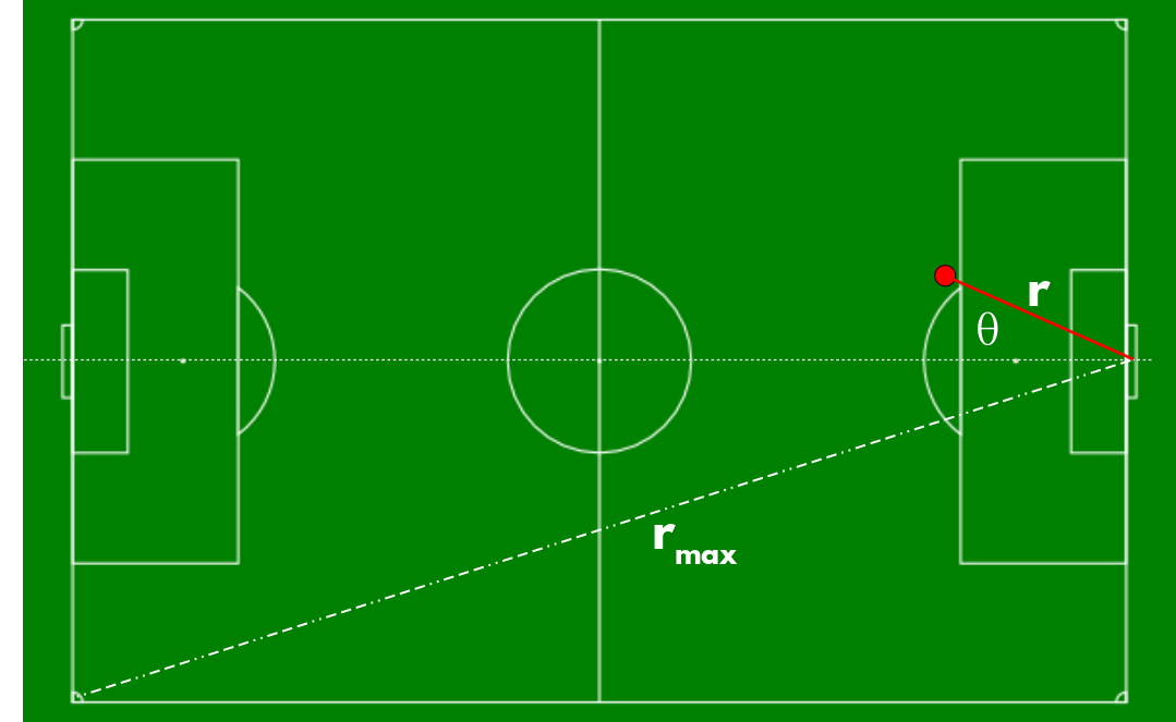
Spatial schematic of a shot (red dot) toward goal in football. Distance is measured from centerline that intersects the two goallines.
Distance: A shot closer to goal has a greater chance of being converted, and a lower chance of being saved, than one further away, but the position of the goalkeeper matters. (And unless one has access to positional data, it won’t be possible to know goalkeeper position.) Distance is measured from shot coordinate to the center of the goal line and normalized by the distance \(r_{max}\) between that point and the far corner so that the rescaled distance is between 0 and 1.
Field Angle: It makes sense that the field angle θ of the shot has an effect on the likelihood of a save. I define this as the angle between the distance vector and the centerline intersecting the two goal lines, and positive angles are shots from the shooting team’s left flank. Then the angle is scaled by \(\frac{\pi}{2}\) so that it lies between -1 and 1.
The next two parameters are defined by the straight path between the shot attempt position and the three-dimensional position in the goalmouth plane that it intersects.
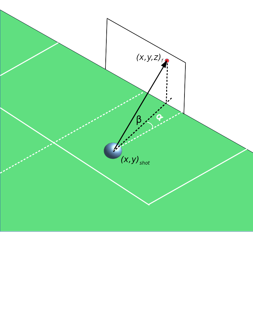
3D schematic of a shot on goal in football. Red dot represents spot where ball crosses goalmouth plane, and alpha and beta are the azimuth and elevation angles, respectively.
Path Azimuth Angle: The angle α of the shot path relative to an (invisible) line that starts at the shot location and intersects perpendicular to the goalline. A positive angle represents a shot toward the opponent’s right post. The angle is scaled by \(\frac{\pi}{2}\) so that it lies between -1 and 1.
Path Elevation Angle: The angle β of the shot path relative to the playing surface. This angle is almost always positive, but can be negative in situations where a ball is headed downwards. It’s scaled by \(\frac{\pi}{2}\) so that it lies between -1 and 1.
Play Type: There are certain events that are more likely to produce goals than others, but the usefulness of this feature depends on the richness of the event data. Some data sets describe shots as the result of set-pieces or throughballs or crosses. Other sets do no more than differentiate open play shots from penalties. The time between play type and the shot can be useful as its own parameter, but it may not always be available.
Body Type: The body part used to execute the shot (and no, hands do not count). I believe that body part could be proxy for shot velocity, and certain body parts are more likely to be used from specific plays (headers from crosses or corners, for example). Again, some data companies include this data but others don’t. I know of a few companies that only describe headed goals but not all headed shots. So this parameter is regrettably optional for some types of data.
Match Time: This variable was present in the expected goals model but I left it out of the expected saves model. My expectation was that shot quality, and therefore shot difficulty to the goalkeeper, had little to do with the time of the match.
Match State: Another variable present in the expected goals model but not in the expected saves model. My expectation here is that a shot is no more difficult to the goalkeeper if the team is tied, up a goal, or down three. (There could be a psychological effect being captured here.)
Other variables: There are a few more variables that I’d like to incorporate if I had years of tracking data, such as goalkeeper position (distance and angle) relative to shot taker and position of closest defender relative to shot taker. I’d like to think that these variables would provide more predictive power to the model, but I’d have to test that.
An alternative Expected Saves model
Another way to estimate xS, which is what I believe most of the analytics community is doing already, is to calculate xG for shots on goal and subtract the sum of those xGs from the total shots on goal. Now we’ve guaranteed that the expected saves model is a complement of the expected goals model for all shots on target.
Training xS models
Expected saves models, like expected goals models are logistic regression models, so I train both models the same way. I described my procedure in my post on expected goals, but if you want to know the basic outline it’s this:
- Scikit-learn‘s LogisticRegression class to create my xG model
- Training, validation, and testing data sets, partitioned by matches
- Brier score as my evaluation metric on the validation data set
One thing that makes xS models challenging than xG models is that there is much less data available to train. While xG models take into account all attempted shots, xS models only consider shots on goal, which reduces the number of data points by 30-40 percent. One can overcome this problem by collecting more data, but that’s not always an option if you don’t work for a data company. It would be useful to run a bias-variance study as a function of the amount of data points in a trained xS model. Come to think of it, such a study would be useful for xG models as well.
To be continued
I would put some evaluation graphics here, but with the new season of Argentina’s Superliga fast approaching, I want to apply this model to last season’s match data first and run some model evaluations later. I will say that the expected saves model gives results that are optimistic — it inflates the number of saves — but are much more believable than an expected saves model based on xG. More about this later.
