Everybody else is doing it, so why can’t we? Soccermetrics’ foray into expected goals
Categories: Goalscoring Models
Expected goals has become a thing — some might say, the thing — in soccer analytics over the last 3-4 years. It is the one metric that has broken out of analyst circles and discussion groups into the football mainstream, and it seems that every analyst has their own expected goals (xG) model that they use to build narratives around certain strategies, players, and teams. It is also the metric that Soccermetrics has been silent about since it reached critical mass.
Well… not really.
I wrote about the idea of expected goals way back in my first Soccermetrics post in January 2009:
I believe that a useful statistic in soccer will ultimately contribute to what I call an “expected goal value” — for any action on the field in the course of a game, the probability that said action will create a goal. One might obtain certain types of data from actions associated with the various positions…
—“Moneyball and soccer”, January 8, 2009
Of course, writing about an idea is one thing; actually implementing it is another. I did some internal work in 2011 on goal probabilities given certain features that are used in xG models, set it aside, and then got swamped by other priorities. In the years since, analysts such as Michael Caley, Sander Ijtsma, and the guys at American Soccer Analysis have taken the lead on developing and disseminating xG models and they deserve the credit and attention that they have gained.
It’s past time for me to get involved in expected goal models and their applications. Since 2011 I have accumulated a lot more practical knowledge about statistics, data modeling, and machine learning that can be used to build useful models to apply to interesting football questions. I don’t expect to write anything ground-breaking in this post; the objective here is to write my modeling methodology down so that I can refer to it and build from it later. If this post turns out to be useful to you, that’s great, too. I do plan on making my code publicly available in short order so that you can tell me how I’m building xG models wrong.
The problem of data
Expected goals models, like all statistical models, depend on data in order to hypothesize about the world. They require large and sufficiently rich data sets to describe and predict the outcomes of shots in a football game. There are sports data companies that provide finely-grained event data — not just temporal and spatial data, but descriptions about the play, the body part used, even the amount of defensive pressing. Other companies may not offer more than the time, spatial coordinates, and a few event flags (was it a penalty? an own goal? a free kick?). It takes hundreds of thousands of shots over multiple seasons to observe meaningful patterns, and obtaining years of such data for modeling is expensive and infeasible.
Last year I asked this question on Twitter…
Is there a public repository of training/testing data that people can use to build and evaluate xG models?
— Soccermetrics (@soccermetrics) July 12, 2016
…and I got some interesting responses. I was referred to Chris Long’s soccer analytics repository on GitHub that contains a huge collection of data from competitions around the world. It’s a massive data set to be sure, not as rich as data from the major sport data companies, but it is one that can be used to build and benchmark expected goals models. So in order to exploit this data set, one has to revisit the question, “At its core, what is an xG model made up of anyway?”
What is an Expected Goals model?
An expected goals model is a conditional probability model that answers the question, “Given a collection of parameters that describes a shot toward goal, what is the probability that a goal is scored?”
Let’s say that \(\mathbf{x}\) represents this collection of parameters (the parameter vector), and \(G\) the goal event. Then we can write this conditional probability model as
\[
Pr(G|\mathbf{x}) = f(\mathbf{\beta}, \mathbf{x})
\]
where \(\mathbf{\beta}\) represents the model coefficients associated with the shot parameters.
Shots are binary events whose probability of success has to be between 0 and 1, which makes a logistic function a great representation. Now the model becomes
\[
Pr(G|\mathbf{x}) = \frac{1}{1 + e^{-\mathbf{\beta}^T\mathbf{x}}}
\]
What are the shot parameters?
It’s the selection of the shot parameters that makes every analyst’s xG model unique as a product of observation, conjecture, and judgment. Some parameters are common to almost all models, but more exotic ones depend on the richness of the data set and the willingness to search the entire possession chain and confirm that a shot occurred within 10 seconds after gaining possession in the final third, executing a through pass, and making a pirouette before curling his shot around the keeper.
I’ve decided to keep the parameters simple for a couple of reasons: to accommodate the limitations of some of the data sets I’ve been working with, and to figure out which parameters are essential.
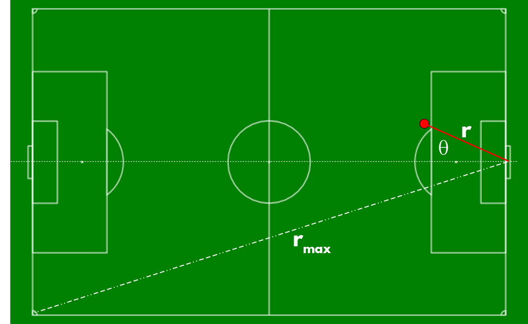
Spatial schematic of a shot (red dot) toward goal in football. Distance is measured from centerline that intersects the two goallines. (Offensive play is from left to right.)
Distance: This is a no-brainer — stands to reason that a shot closer to goal has a greater chance of being converted than one further away. Distance is measured from shot coordinate to the center of the goal line and normalized by the distance \(r_{max}\) between that point and the far corner so that the rescaled distance is between 0 and 1.
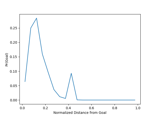
Probability of goal as function of normalized shot distance. Penalties and own goals ignored. Data from Primera División Argentina matches in seasons 2007-2014. Source: Christopher Long
Angle: Another obvious parameter. Again, it stands to reason that shots near the front of goal have a greater chance of being converted. I define this as the angle between the distance vector and the centerline intersecting the two goal lines, and positive angles are shots from the shooting team’s left flank. Then the angle is scaled by \(\frac{\pi}{2}\) so that they lie between -1 and 1.
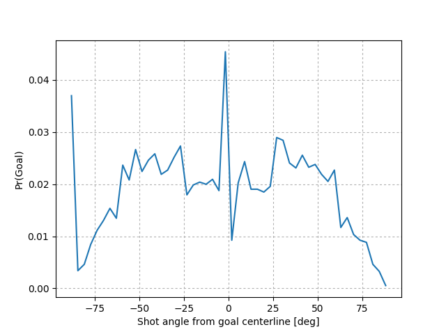
Probability of goal as function of shot angle. Penalties and own goals ignored. Data from Primera División Argentina matches, seasons 2007-2014. Source: Christopher Long
Score/Match State: This parameter was not so obvious to me when I worked on an xG model five years ago, but I’ve been impressed with how significant this parameter is in trained models. Match state is the score differential with respect to the shooter’s team, so if team A leads team B 2-0 and a player from team B makes a shot, the match state is -2. I’ve scaled the match state with a logistic function so that the result is between -1 and 1:
\[
\Delta’ = \frac{2}{1 – e^{-\Delta}} – 1
\]
Match Time: This parameter was not obvious to me either, but I’ve seen it have an effect in other xG models. How much of one is worth discussing but I’ve left it in the model. As you can tell, scaling and normalizing parameters is a big deal for me and time is treated no differently. Shot times are scaled by the duration of the period in which it occurs, so that halftime is always 0.5 and full time is always 1.0. I’m only considering 90 minute matches, but I guess that matches that go to extra time will see match time scaled to 2.0.
Play Type: There are certain events that are more likely to produce goals than others, but the usefulness of this feature depends on the richness of the event data. Some data sets describe shots as the result of set-pieces or throughballs or crosses. Other sets do no more than differentiate open play shots from penalties. The time between play type and the shot can be useful as its own parameter, but it may not always be available.
Body Type: The body part used to execute the shot (and no, hands do not count). I believe that body part is proxy for shot velocity, and certain body parts are more likely to be used from specific plays (headers from crosses or corners, for example). Again, some data companies include this data but others don’t. I know of a few companies that only describe headed goals but not all headed shots. So this parameter is regrettably optional for some types of data.
Competition/Country: It’s easy to believe that “football is football” and that certain shots have a much better chance of going in no matter what the competition. But it seems clear from observation that shot conversion rates depend on the quality and characteristics of the competition. One can choose to capture this in a competition variable (which I believe Michael Caley does) or create individual models for each competition. The advantage of using a competition/country feature is that more training data is available, but the risk is smearing together the individual league characteristics.
Training xG models
I’ve written my own code to implement logistic regression models before, which has its own advantages, but it’s best to use off-the-shelf tools that have already been tested and optimized. To this end, I use the LogisticRegression class from scikit-learn to create my xG model.
For a single competition, I train my model with shot data from matches across multiple seasons. I hold out data from one or two seasons as an out-of-sample set that the model will never see. I then partition the remaining data into a training data set (which yields the parameters) and a validation set (which evaluates the model’s performance) in a 75/25 split. The training/validation data are partitioned at a match level — all of the shots for a particular match are either in the training data set or the validation data set. Scikit-learn has some nice tools that will partition a large dataset into folds that preserve the distribution of successful and unsuccessful shots.
I know that R2 is a popular metric for evaluating the quality of the xG model. I’m not convinced that R2 is a proper metric to use here as the coefficient will rise with the addition of more features in the model and is ultimately a misleading metric. It may still be a good evaluation metric to use, but I’ve been drawn to the Brier score, which is a comparison between predicted probabilities and the actual outcome. I use the Brier score to tune models during cross-validation by comparing predicted goal probabilities to the actual outcomes of shot events. I did a quick search and was pleased to find out that I wasn’t the only one who thought of Brier scores in xG modeling — see SciSports and Pinnacle Sports (although you’re not supposed to use Brier scores for non-binary outcomes).
Demonstration: Primera División Argentina
I first demonstrate the xG model on Argentina’s Primera División over two seasons — a 30-match single round-robin season (plus a derby round) in 2015, and a “transitional” tournament in 2016 in which the teams were split into two groups and they played 15 intragroup matches and one intergroup match (the derby match, usually). I wanted to verify that I could observe the same things as everyone else who had been working with xG models.
This analysis uses a “simple” xG model — body part information is not included in the shot data, and the only plays that we have knowledge of are open play events and penalties.
The relationship between expected and actual goals scored is stronger in the 2015 season than the 2016 season. It could be because of the change in tournament format over the two seasons – half as many games are played in the 2016 transitional tournament. It’s something to explore at a later time.
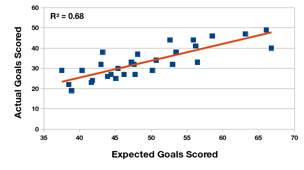
Relationship between expected and actual goals scored, Primera División Argentina 2015 championship.
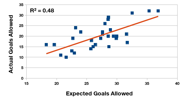
Relationship between expected and actual goals allowed, Primera División Argentina 2015 championship.
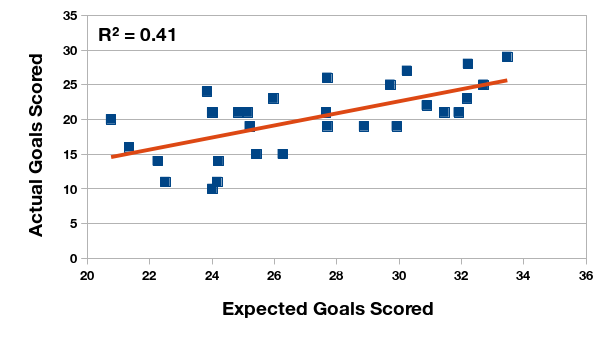
Relationship between expected and actual goals scored, Primera División Argentina 2016 championship.
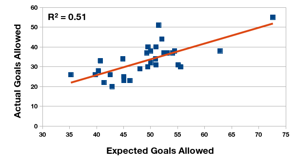
Relationship between expected and actual goals allowed, Primera División Argentina 2016 championship.
One of the characteristics of the xG metric touted by its proponents is its stability over consecutive seasons. In other words, the ratio between expected goals scored and the sum of expected goals scored and allowed is a more robust indicator of a team’s strength than points per game. To test this I computed the points per game and expected goals ratio of the 28 Argentine clubs that competed in the 2015 and 2016 tournaments. The year-on-year relationship between xG ratios in consecutive seasons is a moderately strong one (and this could be a product of the squad and management volatility in the local clubs), but much stronger than a similar relationship between PPG in consecutive seasons.
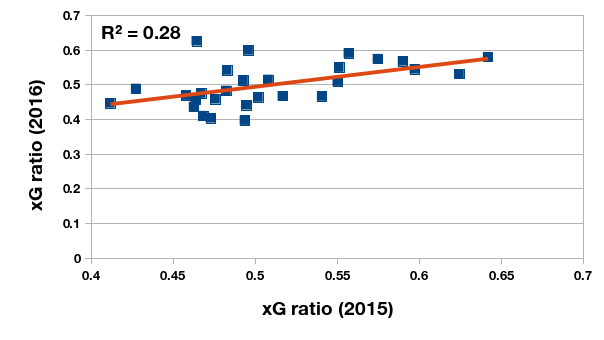
Relationship between xG ratios of Primera División Argentina clubs in 2015 and 2016 championships.
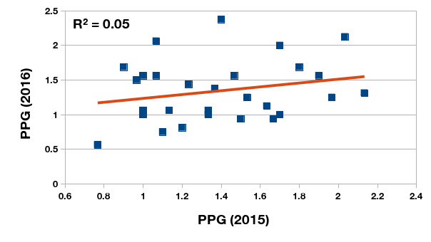
Relationship between points-per-game of Primera División Argentina clubs in 2015 and 2016 championships.
Finally I take a page from Sander’s blog and recreate his predictive quality comparison of popular analytics ratios to the xG ratio. I compare the following metrics: points per game, goal ratio, Total Shot Ratio (shots toward goal), and xG ratio. The plots communicate the correlation between these metrics computed for each team before a given matchday and the same metric computed after the given matchday. In the 2015 tournament the predictive ability of expected goals is stronger than that of TSR, but is consistently below that of goal ratio and points per game in the first half of the season. The 2016 tournament has the really interesting results — the predictive performance of the xG metric lags behind all other metrics. I don’t have any idea why that might be the case (short tournament? group format?), but this definitely falls in the “hey, that’s weird” observation that spurs so much discovery.
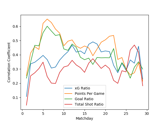
Comparison of predictive quality of Total Shot Ratio, goal ratio, points per game, and xG ratio in Primera División Argentina 2015 championship.
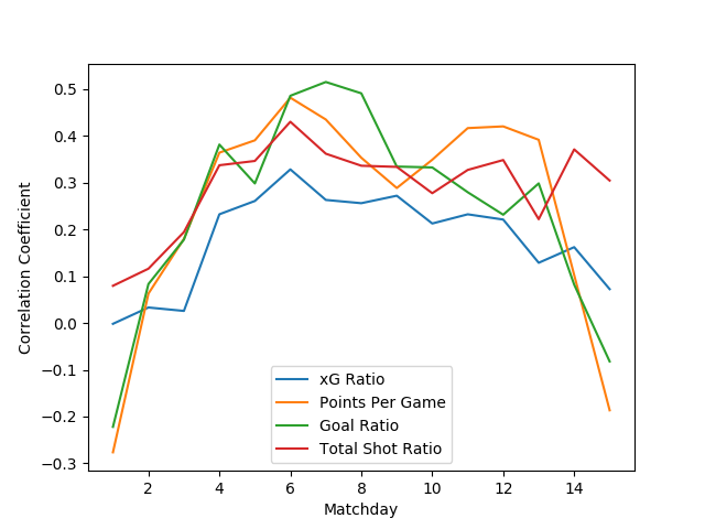
Comparison of predictive ability of Total Shot Ratio, goal ratio, points per game, and xG ratio in Primera División Argentina 2016 championship.
Conclusions
There is so much more to say about expected goals, but this post is almost 2500 words so it’s best to wrap it up. Expected goals is a concept that is here to stay in football analytics. Furthermore, analysts have extended the concept to other plays in soccer, from assists to saves to passes and even defensive actions. I believe that expected goals are capturing some real underlying characteristics of team performance, but it’s not a bulletproof metric (none are) so understanding the idiosyncrasies of the competitions still matters to some degree. Expected goals does deserve its place in the toolbox of football analytics, and now that I’m caught up, I plan on using it more.
